Dynamic Programming(DP) in reinforcement learning refers to a set of algorithms that can be used to compute optimal policies when the agent knows everything about its surroundings; i.e. the agent has a perfect model of the environment. Although dynamic programming has a large number of drawbacks, it is the precursor to almost every other reinforcement learning algorithm. This makes knowing DP a necessity in understanding reinforcement learning. With that said, let’s begin.

Dynamic Programming - A Brief Introduction

For those of you who know what dynamic programming is, feel free to skip this subsection.

Dynamic programming, for the uninitiated, is reusing previously calculated values to compute the next value. Suppose we have to find the answer of $2 \times 2 \times 2$ and $2 \times 2 \times 2 \times 2$ . By calculating $2 \times 2 \times 2 = 8$ first, we can be reuse it - $2 \times 2 \times 2 \times 2 = 8 \times 2 = 16$ - to reduce the total number of multiplications. This makes problems that would otherwise grow exponentially with size to become polynomial - a major speed-up. In real terms, problems that may take over an hour to solve naively can be done in seconds.

We perform dynamic programming by storing previously calculated values in a table. There are two main techniques of dynamic programming: tabulation and memoization. Both methods have their pros and cons. GeeksForGeeks has a whole series on dynamic programming, which goes in-depth into the topic.

The Theoretical Jargon

To my utter dismay, we can’t proceed with this article without theory. Dynamic programming in RL has strict conditions we need to adhere to, which includes a lot of theory.

Markov Decision Process (MDP)

In the very first line of the article I’ve said that dynamic programming requires a perfect model of the environment. But what does this perfect model really mean?

In our case, a perfect model means the agent has access to the likelihood of every action happening. The actions themselves must remain the same. Moreover, the probability of the agent moving from state s to state s' is conditionally independent - if the action takes place at time t it only depends on the probabilities at time t-1. The process is “memoryless”. The representation of the action space is a type of probability matrix a known as a Markov Chain.

The importance of conditional independence may not be inherently obvious. An example of such independence would be in population growth. One only needs to know the current population and rate of natural increase(birth rate - death rate) to estimate the future population. Old data is not required. On the other hand, if you go to the doctor with a cough and chest pain, the doctor won’t just look at your current state and give you a prescription. He or she will have to look at your medical history. Prior data is a must.

In terms of reinforcement learning, conditional independence simplifies much of the mathematics involved. If the agent had to take all his previous actions into consideration each time it took a new one, training would take forever. And while many processes may not satisfy this Markov property, working under that assumption usually leads to accurate results.

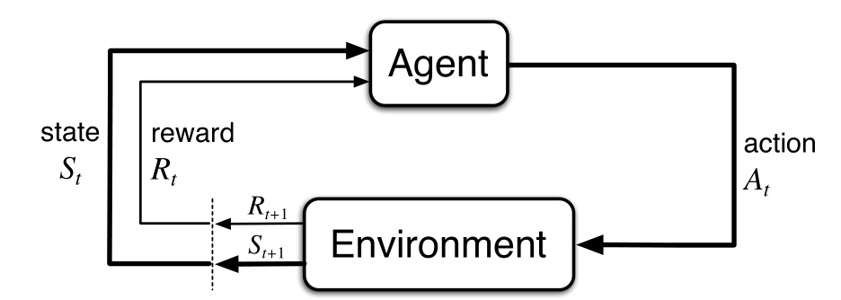
A reinforcement learning problem that satisfies this Markov property is called a Markov Decision Process. A finite task is one that has a clear beginning and ending, i.e. there is a known number of possible states and actions. If the task is finite, the problem becomes a finite MDP. The agent interacts with the environment and receives feedback in the form of a reward. At each time step t, the environment changes due to the agent’s action. These changes are represented by the changing values in the Markov chain.

The Agent Environment Interaction Diagram. Source: Sutton & Barlo

The Value Function

In reinforcement learning problem, our objective boils down to estimating the value of states (or of state-action pairs¹). The agent’s mapping of individual states to numbers is known as the value function. This value indicates “how good” a state is in terms of expected future reward.

In practical terms a value function is a list of numbers: each number corresponding to the preference of a particular state. The process of refining the value function to reach the optimal policy is what dynamic programming is all about.

Discounting - Not all rewards are created equal

By definition, the value of a state is its long-term reward potential. At time t, we need to consider the rewards of the states from time t+1 to the end of the episode. But now a new question arises. How should we differentiate between an instanteneous reward with one that is further into the future? Depending on the task, we may choose to prioritize short-term rewards over long-term ones. The way we do this is by a process called discounting. The expected² discounted reward at time t, $G_t$ is

$G_t = R_{t + 1} + \gamma R_{t + 2} + \gamma^2 R_{t + 3} + \cdots = \sum_{k=0}^{\infty}\gamma^k R_{t + k + 1}$

$\gamma$ ( $0 \leq \gamma \leq 1$ ) is known as the discount rate. $R_t$ is the reward received at time t.

The discount rate ensures that further the reward, the less is it is valued. This is particularly important if each episode is very long or infinite (the continuing task case). If we set $\gamma = 0$ , the agent becomes myopic, only seeking to maximize the immediate reward at all times. In tasks such as pole balancing (the CartPole environment), a myopic strategy works perfectly well. And as $\gamma$ approaches 1, the agent becomes more far-sighted. As long as the discount rate is less than 1, the infinite sum is bound to converge.

Bellman Equations

Bellman optimality equations, or Bellman equations, are a set of equations defining the relationship between the value of a state and the value of its successor states. Solving this system of equations for a reinforcement learning task gives us the optimal value function.

For the optimal policy $\pi_*$ and an arbitrary state s, the optimal value function $V_{*}$ under the Bellman optimality equation is

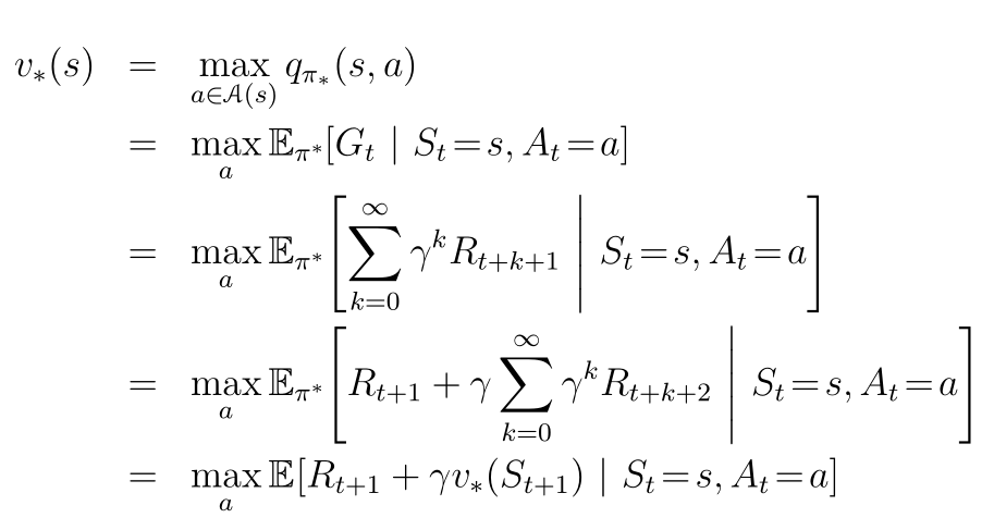
Yes, the equation looks terrifying, but what it says is relatively straightforward: the value of a state under an optimal policy must equal the expected return for the best action from that state. At a state s, we choose the action a that gives the maximum reward $R_{t + 1}$ plus the discounted reward from the next state $\gamma V_{*}(S_{t + 1})$ .

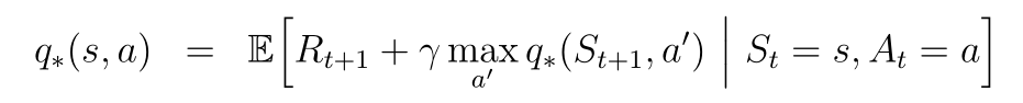
The Bellman optimality equation for the optimal state $s_{*}$ is similar, only here we know the best action.

Finding the inverse of the Markov chain will result in the solution of the Bellman equation for the value function. However, inverting a matrix is a slow, computationally expensive task. Dynamic programming algorithms attempt to find a good approximation to this inverse.

Don’t worry too much if you don’t completely understand this subsection. The implementation is simpler than the equation.

Walking on a FrozenLake

We will now go through and implement the dynamic programming algorithms on OpenAI Gym’s FrozenLake-v0 environment.

The FrozenLake

OpenAI’s FrozenLake environment is a 4 by 4 or 8 by 8 grid representing an icy lake. The goal here is to go from the starting position S to the finish F while avoiding the holes H. The lore is as follows:

Winter is here. You and your friends were tossing around a frisbee at the park when you made a wild throw that left the frisbee out in the middle of the lake. The water is mostly frozen, but there are a few holes where the ice has melted. If you step into one of those holes, you’ll fall into the freezing water. At this time, there’s an international frisbee shortage, so it’s absolutely imperative that you navigate across the lake and retrieve the disc. However, the ice is slippery, so you won’t always move in the direction you intend. (Source: OpenAI)

env = gym.make("FrozenLake-v0") 
env.reset()
env.render()
>>> SFFF            # (S: start)
    FHFH            # (F: frozen, safe)
    FFFH            # (H: hole, failure)
    HFFG            # (G: goal)

There are 16 possible positions the agent can be on, i.e. 16 possible states. The agent can take 4 actions: LEFT(0), DOWN(1), UP(2) and RIGHT(3).

num_states = env.observation_space.n
num_actions = env.action_space.n
print(num_states, ", ", num_actions)
>>> 16, 4

The special factor about this environment is that the agent often does not do what we tell it to. I demonstrate this below

state = env.reset()
print(state)
>>> 0        # Starting position
# Let's make the agent go a step downwards
new_state, reward, is_done, info = env.step(1)  
print(new_state)  
>>> 1       # The agent went to the left instead
print(reward)
>>> 0     

The agent went the other way instead. Let’s print the info variable to see the reason.

print(info)
>>> {'prob': 0.3333333333333333}

The probability of the agent performing a particular action is 1/3. Not the easiest environment to traverse. The reward is 1 at the goal, and 0 everywhere else. This makes the environment impossible for the random search algorithm to solve. Feel free to try it out on your own. I personally found my agent successfully traversing FrozenLake less than 15% of the time (given 1000 attempts).

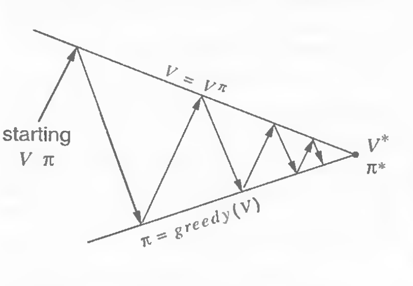
Iteration: Evaluation and Improvement

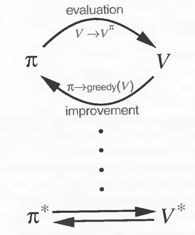
Iteration, evaluation, and improvement were things I often mixed up when I first started learning this topic. We evaluate policies. By this I mean that for a new policy, we update our value function based on the new action taken and the previous set of values. This update process follows the Bellman Optimality Equation for the value function.

After we have our updated values, we use this to improve our policy. This is done by choosing the actions that have the highest updated values (greedy). The equation used here is the Bellman Optimality Equation for the optimal state.

Now that we have a new policy, we evaluate this policy again. This cyclic process is known as iteration. Starting with arbitrary value and policy functions, the iteration process leads us to the optimal $V_{*}$ and $\pi_{*}$ sooner or later.

Policy improvement cycle	The goal of policy improvement

Policy Evaluation

Firstly let’s go through the policy evaluation algorithm. The task here is to compute the value function for the policy π using the Bellman equation. The value function is computed iteratively, that is, we repeatedly keep running the equation until the function converges (the difference is less than a threshold value).

Before we start, there is one aspect to this algorithm (and the subsequent ones) that make it a dynamic programming algorithm. That is complete environment knowledge. In toy problems this knowledge of action probabilities is often called the “transformation matrix”. As for the FrozenLake environment, this is how we access it.

from pprint import pprint  # Cleaner print formatting
# Let's print the action probabilities at position 0
pprint(env.env.P[0])
>>> {0: [(0.3333333333333333, 0, 0.0, False),
     (0.3333333333333333, 0, 0.0, False),
        (0.3333333333333333, 4, 0.0, False)],
    1: [(0.3333333333333333, 0, 0.0, False),
        (0.3333333333333333, 4, 0.0, False),
        (0.3333333333333333, 1, 0.0, False)],
    2: [(0.3333333333333333, 4, 0.0, False),
        (0.3333333333333333, 1, 0.0, False),
        (0.3333333333333333, 0, 0.0, False)],
    3: [(0.3333333333333333, 1, 0.0, False),
        (0.3333333333333333, 0, 0.0, False),
        (0.3333333333333333, 0, 0.0, False)]}

env.env.P is a dictionary where the keys are states and values are dictionaries of possible actions and their outcomes. Each action has a probability of 1/3 of happening, the next value represents the resulting position the agent might land on (it can go to either to the right - 1 - or down - 4). The 3rd value is the reward for that action which is 0 everywhere except the goal. The final value is a boolean that indicates whether the episode ends as a result of that action. This happens when the agent reaches the goal or falls into a hole. Now let’s look that the probabilities at position 5, a hole.

# Let's print the action probabilities at position 5
pprint(env.env.P[5])
>>> {0: [(1.0, 5, 0, True)],
    1: [(1.0, 5, 0, True)],
    2: [(1.0, 5, 0, True)],
    3: [(1.0, 5, 0, True)]}

Once the agent has fallen into a hole, it can’t get out. The episode terminates. There is no reward. When approaching the goal, for example in position 14, some outcomes have a reward of 1. Feel free to look at other positions to see what their outcomes are.

Getting back to the topic, I will first write down the function and then we can go through it in parts.

threshold = 0.0001      # convergence threshold
gamma = 0.99            # discount rate

The two parameters we set are the discount rate and convergence threshold. The threshold defines a stopping point for the function. The smaller the threshold, the more accurate the values, but the longer the time taken to converge. A gamma of 0.99 is suitable for this environment, but feel free to try out different values and see what works best.

def policy_evaluation(env, policy, gamma, threshold):
    num_states = env.observation_space.n
    V = torch.zeros(num_states)
    max_delta = threshold + 1
    while max_delta > threshold:
        temp = torch.zeros(num_states)
        for state in range(num_states):
            action = policy[state].item()
            for proba, new_state, reward, _ in env.env.P[state][action]:
                temp[state] += proba * (reward + V[new_state] * gamma)
        max_delta = torch.max(torch.abs(V - temp))
        V = temp.clone()
    return V

We first define our value array V as a 1D matrix of 0s. max_delta stores the maximum difference in value for a state between two consecutive iterations. We use this to check for convergence. temp is the new value function that is temporary defined as another 1D matrix of 0s.

for state in range(num_states):
    action = policy[state].item() # item() converts Tensor to int

For each state, we choose the action specified by the policy function.

for proba, new_state, reward, _ in env.env.P[state][action]:

As we have seen before, P is a dictionary of dictionaries. We are taking the possible actions in P[state] and then iterating through the possible outcomes for an action in P[state][action].

temp[state] += proba * (reward + V[new_state] * gamma)

The value function for a state is the expected sum (+= proba *) of the reward (reward + ) and discounted future rewards (V[new_state] * gamma).

max_delta = torch.max(torch.abs(V - temp))

This line computes the maximum absolute difference between the value function at the current iteration temp against the value function at the previous iteration v. V = temp.clone() simply copies the new value function onto the old one.

If you have understood everything up to this point, rejoice! We are almost at the finish line.

Policy Iteration

Policy iteration consists of policy evaluation and policy improvement. Now that we are done with policy evaluation, the next step in this cycle is policy improvement.

def policy_improvement(env, V, gamma):
    num_states = env.observation_space.n
    num_actions = env.action_space.n
    policy = torch.zeros(num_states)
    for state in range(num_states):
        actions = torch.zeros(num_actions)
        for action in range(num_actions):
            for proba, new_state, reward, _ in env.env.P[state][action]:
                actions[action] += proba * (reward + V[new_state] * gamma)
        policy[state] = torch.argmax(actions)
    return policy

Here, we set our policy function to a matrix of 0s.

for state in range(num_states):
    actions = torch.zeros(num_actions)

A matrix of 0s corresponding to the available actions is initialized.

for action in range(num_actions):
    for proba, new_state, reward, _ in env.env.P[state][action]:
        actions[action] += proba * (reward + V[new_state] * gamma)
policy[state] = torch.argmax(actions)

This is part of the Bellman optimality equation for the policy function. The value of each action at the given state is updated by the expected current reward and the discounted future reward. After the value of each action at the given state is calculated, the action with the highest reward is selected using torch.argmax(actions).

The policy iteration algorithm alternates between these two functions until the optimal policy is reached.

def policy_iteration(env, gamma=0.99, threshold=0.0001):
    num_states = env.observation_space.n
    num_actions = env.action_space.n
    policy = torch.randint(high=num_actions, size=(num_states,)).float()
    while True:
        V = policy_evaluation(env, policy, gamma=gamma, threshold=threshold)
        new_policy = policy_improvement(env, V, gamma=gamma)
        if torch.equal(new_policy, policy):
            return V, new_policy
        policy = new_policy.clone()

Using torch.randint() we create an arbitrary policy of random numbers (in the range 0, num_actions). We keep running the policy evaluation -> policy improvement loop until there is no improvement in our policy torch.equal(new_policy, policy).

V_optimal, optimal_policy = policy_iteration(env)
total_reward = []
for n in range(NUM_EPISODES):
    total_reward.append(run_episode(env, optimal_policy))
print(f"Success rate over {NUM_EPISODES} episodes: {sum(total_reward) * 100 / NUM_EPISODES}%")
>>> Success rate over 1000 episodes: 84.3%

As we can see, policy iteration has a tremendous success rate (84.3% vs <15%) over the random strategy.

Policy iteration is particularly useful when we already know a starting policy, i.e. we know a decent strategy to solve the problem. In addition, if the environment has a large number of possible actions, this method converges faster than value iteration.

Value Iteration

Value iteration is similar to policy iteration. But where policy iteration uses the Bellman optimality equation for the policy function, value iteration uses it for the value function. This method is marginally better when there are fewer actions to deal with.

def value_iteration(env, gamma=0.99, thres = 0.0001):
    num_states = env.observation_space.n
    num_actions = env.action_space.n
    V = torch.zeros(num_states)
    max_delta = thres + 1
    while max_delta > thres:
        temp = torch.zeros(num_states)
        for state in range(num_states):
            v_actions = torch.zeros(num_actions)
            for action in range(num_actions):
                for proba, new_state, reward, is_done in env.env.P[state][action]:
                    v_actions[action] += proba * (reward + gamma * V[new_state])    # Value iteration 
            temp[state] = torch.max(v_actions)              # Select the action with the highest reward
        max_delta = torch.max(torch.abs(V - temp))
        V = temp.clone()
    return V

As you can see, this algorithm is very similar to that of policy evaluation. There are some major differences.

temp = torch.zeros(num_states)
for state in range(num_states):
    v_actions = torch.zeros(num_actions)
    for action in range(num_actions):
        for proba, new_state, reward, is_done in env.env.P[state][action]:
            v_actions[action] += proba * (reward + gamma * V[new_state])
    temp[state] = torch.max(v_actions)

Instead of selecting an action from a given policy, we calculate the values of all policies using the value matrix of the previous iteration and then choose the greatest calculated value as the value of that state. This is the Bellman optimality equation for the value function, stripped of all of its mathematical illegibility. v_actions[action] += proba * (reward + gamma * V[new_state]) calculates the expected value for each state, while temp[state] = torch.max(v_actions) greedily selects the max value from the matrix of action values.

Extracting the optimal policy here is exactly the same as the policy improvement function. I am including it here separately for completeness.

def extract_optimal_policy(env, V, gamma=0.99):
    num_states, num_actions = env.observation_space.n, env.action_space.n
    optimal_policy = torch.zeros(num_states)
    for state in range(num_states):
        v_actions = torch.zeros(num_actions)
        for action in range(num_actions):
            for proba, new_state, reward, _ in env.env.P[state][action]:
                v_actions[action] += proba * (reward + gamma * V[new_state])
        optimal_policy[state] = torch.argmax(v_actions)
    return optimal_policy

optimal_values = value_iteration(env)
optimal_policy = extract_optimal_policy(env, optimal_values)
total_reward = []
for n in range(NUM_EPISODES):
    total_reward.append(run_episode(env, optimal_policy))
print(f"Success rate over {NUM_EPISODES} episodes: {sum(total_reward) * 100 / NUM_EPISODES}%")
>>> Success rate over 1000 episodes: 87.3%

Value iteration does 3% better than policy iteration here, and is slightly faster to train.

Conclusion

Dynamic programming uses complete environment knowledge to accurately compute optimal values and policies with straightforward methods. The methods used go through all possible actions and futures in each state, doing what is known as full backups. It goes without saying that this is not the most efficient way of doing things. Moreover, this makes DP methods not scale to larger problems; DP specially struggles in problems with a large number of states.

Policy evaluation iteratively computes the value function for a given policy, while policy improvement calculates an improved policy from a given value function. These methods combine to form policy and value iteration, the main DP algorithms.

DP uses estimates of future values to estimate the present value. This method of bootstrapping is used in many other reinforcement learning algorithms, namely in temporal difference learning methods.

The next article will focus on Monte Carlo methods, which not just not require full environment knowledge, don’t even need a model of the environment to work. Monte Carlo methods are very efficient and easily scale to large problems.

Footnotes

[1] A state-action pair is the grouping of a state and a particular action into a single value. In a backup diagram, this would be the difference between assigning values to states themselves or to actions (state transitions).

[2] The term expected return is used because we are calculating future rewards, which by nature is uncertain. Therefore, the expected return is a more sensible measure compared to trying to calculating the maximum reward from each state.

Dynamic Programming RL

RL Basics