Previously, we looked into the Monte Carlo family of reinforcement learning algorithms. These methods estimate the solution to a RL problem by learning from experience. Just by simulation and blind exploration, Monte Carlo agent reaches the optimal solution.

Today, we will go through an interesting case: the game of roulette. We will discover the optimal strategy to win at roulette and hopefully close down a few casinos in the process.

The Game

A roulette wheel consists of a spinning disk with divisions around its edge that revolves around the base of a bowl. A ball is spun around the outside of the bowl until eventually ball and wheel come to rest with the ball in one of the divisions. The divisions around the wheel are numbered from 1 to 36 in a seemingly random pattern and alternate red and black. Prior to rolling the ball, people place bets on what number will come up by laying down chips on a betting mat, the precise location of the chips indicating the bet being made¹.

The Player

We will set up the game in OpenAI Gym’s Roulette-v0 environment. Let’s first do the basic imports.

import torch
import gym

The agent (our algorithm) interacts with the environment we create here.

env = gym.make("Roulette-v0")

Our agent will play the game a number of times, each time choosing to either bet on a number or walk away with its winnings. There are 4 sets of possible actions:

• The agent bets on an even number (except 0).
• The agent bets on an odd number.
• The agent bets on 0.
• The agent walks away from the board.

There are 3 possible types of rewards for the agent’s action.

• The rolled number is not zero and its parity matches the agent’s bet -> +1
• The rolled number’s parity does not match the agent’s bet -> -1
• The rolled number and the agent’s parity are both zero -> +36

Betting on a zero is the highest risk, highest reward outcome.

Our agent therefore has 38 possible actions to choose from - the numbers 0 to 36 and walking away (37).

num_actions = env.action_space.n
print(num_actions)
>>> 38

In the roulette simulation, the environment only has one state. This is because a game ends after one action (the bet). This state is denoted by 0.

num_states = env.observation_space.n
print(num_states)
>>> 1
state = env.reset()
print(state)
>>> 0

The outcome for an action can be -1, 1, 0 or 36.

env.step(1)  # Ball lands on odd number
>>> (0, 1.0, False, {})
env.step(1)  # Ball lands on even number / zero
>>> (0, -1.0, False, {})
env.step(0)  # Ball lands on zero
>>> (0, 36.0, False, {})
env.step(37) # Agent walks away
>>> (0, 0.0, True, {})

The game will end if the agent walks away (action 37) or after 100 spins of the wheel/iterations.

The On-Policy Strategy

The first way in which we’ll solve this problem is using on-policy Monte Carlo control. Here we will use the ϵ-greedy approach to update the policy function.

The Simulation

Let’s first start by defining the episode simulating function using ϵ-greedy.

def run_eps_episode(env, Q, epsilon, num_actions):
    state = env.reset()
    memo = []
    is_done = False
    # epsilon-greedy starting probabilities
    proba = torch.ones(num_actions) * epsilon / num_actions    
    while not is_done:
        best_action = torch.argmax(Q[state]).item()
        proba[best_action] += 1 - epsilon
        # Choose 1 action from the multinomial distribution
        action = torch.multinomial(proba, 1).item()               
        
        new_state, reward, is_done, info = env.step(action)
        memo.append((state, action, reward))
        state = new_state
    return memo

The initial probabilities in the ϵ-greedy policy is ϵ/size of the action space: proba = torch.ones(num_actions) * epsilon / num_actions.

Every iteration we update the likelihood of the best action by 1-ϵ: proba[best_action] += 1 - epsilon. The best action is selected from a multinomial distribution (a distribution with many outcomes) using torch.multinomial(proba, 1).

Here we are storing the states, actions, and rewards as a list of triples (state, action, reward). This makes iterating through them cleaner.

The Algorithm

We use first-visit Monte Carlo to evaluate state-action pairs returned from each simulation.

We will use a new data type, the defaultdict to keep track of rewards, frequency and the Q-function. defaultdict is a part of the built-in collections library.

from collections import defaultdict

We have to assign a datatype or structure to defaultdict declarations. This is the default value for any key. For example,

d1 = defaultdict(int)
print(d1[5])
>>> 0

If the key does not exist, it is automatically set to the default value. Similarly,

d2 = defaultdict(lambda: torch.zeros(num_actions))

lambda is an inline function. Here a tensor of zeroes is created for each key. Another function we use here is tqdm. This is a very pleasant wrapper that I highly recommend. Wrap it around a function or a loop and you can see a real-time progress bar.

from tqdm import tqdm

If you don’t already have the library, use pip install tqdm in the terminal. We will see how tqdm works below.

def on_policy_mc_control(env, gamma, epsilon, num_episodes):
    num_actions = env.action_space.n
    G_sum = defaultdict(float)
    N = defaultdict(int)
    Q = defaultdict(lambda: torch.zeros(num_actions)) 
    for episode in tqdm(range(num_episodes)):
        memory = run_eps_episode(env, Q, epsilon, num_actions)
        net_reward = 0
        G = {}
        for state, action, reward in reversed(memory):
            net_reward = gamma * net_reward + reward
            G[(state, action)] = net_reward
        for state_action, net_reward in G.items():
            G_sum[(state, action)] += net_reward
            N[(state, action)] += 1
            Q[state][action] = G_sum[(state, action)] / N[(state, action)]
    policy = {}
    for state, actions in Q.items():
        policy[state] = torch.argmax(actions).item()
    return Q, policy

We first define our dictionaries

G_sum = defaultdict(float)
N = defaultdict(int)
Q = defaultdict(lambda: torch.zeros(num_actions)) 

G_sum records the total rewards through all episodes. N keeps track of the frequency of each state-action pair. A state-action pair is simply the tuple (state, action). Q is the Q-function, the function that keeps track of the value of state-action pairs.

for episode in tqdm(range(num_episodes)):

tqdm shows a progress bar and tells you how long it will take for execution to complete.

memory = run_eps_episode(env, Q, epsilon, num_actions)
net_reward = 0
G = {}
for state, action, reward in reversed(memory):
    net_reward = gamma * net_reward + reward
    G[(state, action)] = net_reward

We initially set the net reward to 0. This is the discounted reward. At each (state, action, reward) tuple, the net reward is updated and stored in G.

for state_action, net_reward in G.items():
    G_sum[(state, action)] += net_reward
    N[(state, action)] += 1
    Q[state][action] = G_sum[(state, action)] / N[(state, action)]

At the end of each episode, we add the values in G to G_sum and increment the frequency counter N by 1 (first-visit MC). We then update the Q-function to the new average.

The benefit of using defaultdict is that we don’t need to check if a key initially exists. The code simplifies from

if (state, action) in N.keys():
    N[(state, action)] += 1
else:
    N[(state, action)] = 1

to

N[(state, action)] += 1

After numerous sample episodes, we approximate the optimal Q function, which in turn translates to the optimal policy.

The Results

Let’s first set our constants. We use a γ=1 because every reward equally affects the net reward, discounting does not make sense.

gamma = 1
epsilon = 0.1
num_episodes = 5000

We can now see the optimal policy for roulette using on-policy MC.

optimal_Q, optimal_policy = on_policy_mc_control(env, gamma, epsilon, num_episodes)
print(optimal_policy)
>>> {0: 37}

So the optimal policy is always betting on 37. But wait, 37 maps to walking away from the table. So the best way to win at Roulette is just not playing at all?

Let’s now look at how results change when the number of episodes is increased.

episode_list = [5000, 50000, 500000]

on_policy_dict = {}
for num_episodes in episode_list:
    optimal_Q, optimal_policy = on_policy_mc_control(env, gamma, epsilon, num_episodes)
    on_policy_dict[num_episodes] = [optimal_Q, optimal_policy]

In each case the optimal policy is still 37. To test our policy, we need to run it in a number of simulations.

def run_test(policy, iters, num_episodes):
    env = gym.make("Roulette-v0")
    rewards = [0] * num_episodes
    wins = 0
    losses = 0
    for i in range(num_episodes):
        state = env.reset()
        is_done = False
        total_reward = 0
        while not is_done:
            action = policy[state]
            state, reward, is_done, _ = env.step(action)
            total_reward += reward
        rewards[i] = total_reward
        if total_reward >= 1:
            wins += 1
        elif total_reward <= -1:
            losses += 1
    label= f"{iters} iterations Win rate: {wins/num_episodes}  Loss rate: {losses/num_episodes}"
    return rewards, label

If the reward is 0 (walking away immediately), it counted as neither a win or a loss. We use the rewards array and label in the graphs below.

To make visual plots, we use the matplotlib library.

import matplotlib.pyplot as plt

matplotlib is a very user-friendly library, and the website provides great tutorials on usage. For now, we will use the plot_roulette function for visualizations.

def plot_roulette(result_dict, title, num_episodes = 1000):
    for k, v in result_dict.items():
        optimal_Q, optimal_policy = v
        plt.plot(np.arange(len(optimal_Q[0])), optimal_Q[0].numpy(), label=f"{k} iterations")
    plt.xlabel("Action")
    plt.ylabel("Action-Value")
    plt.legend()
    plt.title(str.title(title))
    plt.show()
    for k, v in result_dict.items():
        optimal_Q, optimal_policy = v
        rewards, label = run_test(optimal_policy, k, num_episodes)
        plt.plot(rewards, label=label)
    plt.xlabel("Episode")
    plt.ylabel("Reward")
    plt.legend()
    plt.show()

From the on-policy MC results, we see the following.

plot_roulette(on_policy_dict, "on-policy control")

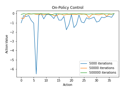
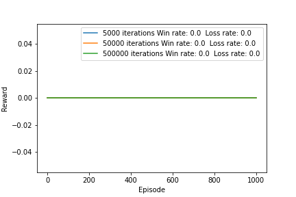
The action-values meet our expectations here. As the number of episodes increase, the action-values converge to -1/37. The action-value for leaving the board is always 0. As for the total rewards, the agent chooses not to play the game.

The Off-Policy Strategy

In off-policy MC control, we use a behavior policy to optimize the target policy π. As for the type of importance sampling, we will use the incremental variant of weighted importance sampling. The incremental variant uses a slightly modified update rule speeding up the process significantly.

The Simulation

For the off-policy simulations, we will follow the random behavior policy to select actions.

def generate_random_policy(num_actions):
    probs = torch.ones(num_actions) / num_actions
    def policy_function(state):
        return probs
    return policy_function

The behavior policy used is very straightforward, giving each action in any state an equal likelihood of being selected. This ensures stochasticity. Moreover, we usually do not know the number of possible states. Each state getting the same probabilities therefore makes sense.

def run_episode(env, behaviour_policy):
    state = env.reset()
    memo, is_done = [], False
    while not is_done:
        probs = behaviour_policy(state)
        action = torch.multinomial(probs, 1).item()
        new_state, reward, is_done, info = env.step(action)
        memo.append((state, action, reward))
        state = new_state
    return memo

Notice that we use behaviour_policy(state) to get a 1D Tensor of probabilities. torch.multinomial(probs, 1) is used to select an action based on the probabilities given.

The Algorithm

def off_policy_mc_contro(env, gamma, num_episodes, behaviour_policy):
    num_actions = env.action_space.n
    N = defaultdict(int)
    Q = defaultdict(lambda: torch.zeros(num_actions))
    for episode in tqdm(range(num_episodes)):
        w = 1.0
        states, actions, rewards = run_episode(env, behaviour_policy)
        net_reward = 0    
        for state, action, reward in zip(reversed(states), reversed(actions), reversed(rewards)):
            net_reward = gamma * net_reward + reward
            N[(state, action)] += w                                # Incremental update
            Q[state][action] += (w / N[(state, action)]) * (net_reward - Q[state][action])   
            if action != torch.argmax(Q[state]).item():
                break
            w = w / behaviour_policy(state)[action]
    policy = {}
    for state, actions in Q.items():
        policy[state] = torch.argmax(actions).item()
    return Q, policy

Due to the incremental update, we do not keep track of rewards, G_sum, instead updating the Q-function in-place. We substitute with . Instead of calculating the Q-function in a for loop in the end, we update it in each iteration. N is the sum of weights for the state-action pair up-to that point.

N[(state, action)] += w
Q[state][action] += (w / N[(state, action)]) * (net_reward - Q[state][action]) 

This time, we need to keep track of a new variable, w, the weight of each state-action pair. As the number of appearances of a state-action pair increases, w increases. This is because the denominator
behaviour_policy(state)[action] . States that appear earlier on are weighed higher.

if action != torch.argmax(Q[state]):
    break

The update process only runs when the target and behavior policies choose the same actions.

The Results

We will use the same γ=1 here.

gamma = 1
episode_list = [5000, 50000, 500000]
random_policy = generate_random_policy(env.action_space.n)

The results this time are awry. As the number of iterations increase, the optimal policy changes, albeit to an incorrect outcome.

off_policy_dict = {}
for num_episodes in episode_list:
    optimal_Q, optimal_policy = off_policy_mc_control(env, gamma, num_episodes, random_policy)
    off_policy_dict[num_episodes] = [optimal_Q, optimal_policy]
    print(num_episodes, ": ", optimal_policy)
>>> 5000: {0: 25}
>>> 50000: {0: 30}
>>> 500000: {0: 1}

We see a similar mess in the plots.

plot_roulette(off_policy_dict, "off-policy control", num_episodes=1000)

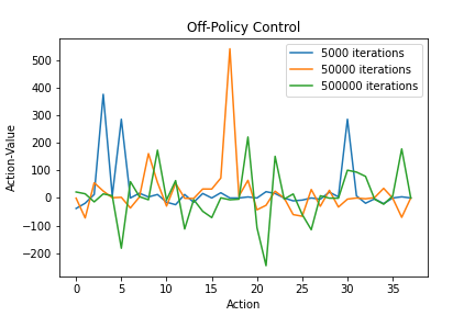
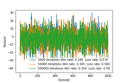
Off-policy Monte Carlo control fails to solve the roulette problem. Running the algorithm gives a different optimal policy each time. My hypothesis is that because off-policy control stops learning from an episode the moment the behavior and target policies differ, whenever the optimal early stopping scenario comes up in the behavior policy sequence, it doesn’t match the target policy. Thus the agent doesn’t learn from that episode. In cases where the first few actions may have a simulation-ending impact, off-policy Monte Carlo control may be unsuitable.

Conclusion

On-policy and off-policy Monte Carlo control algorithms have their strengths and weaknesses. The weakness of the off-policy approach was seen in roulette. On-policy MC is also significantly faster per episode in this environment, taking 69 seconds for 500,000 iterations. On the other hand, off-policy MC required 40 minutes for the same task.

It should be noted that when the agent is not allowed to walk away from the game, both policies converge to the same optimal policy {0:0} -> the agent always bets on the high-risk, high-reward 0. I’ll leave that for you to try out; one just has to prevent action 37 from being selected. In other games like blackjack, off-policy Monte Carlo fares slightly better than its on-policy counterpart (42.4% vs 43.7% win rate²).

So there we have it, Monte Carlo reinforcement learning - a powerful tool. The takeaway from this article - maybe tone down on the little wheel, the only one feeling real lucky is the casino.

Footnotes

[1] Master Traditional Games. Rules of Roulette

[2] This result is from some experiments I ran following Sutton & Barlo’s Reinforcement Learning, An Introduction. This environment is available in the Gym as Blackjack-v0.