Temporal Difference Learning - the holy amalgamation of Monte Carlo and dynamic programming. Taking the best of both worlds, TD learning is a faster, model-less, more accurate method of solving reinforcement learning problems. TD is a concept that was first developed in reinforcement learning, and only later branched to other fields such as computer vision.

Temporal difference learning uses concepts from both MC and DP, while at the same time improving over them. TD methods:

Learn directly from raw experience without a model or environment specifications - Similar to Monte Carlo
Update estimates based on prior estimates without waiting for final outcomes (bootstrapping) - Similar to DP
Use the same General Policy Iteration approach seen in all other methods.
Works well in non-stationary environments (where probabilities change over time).
Estimates are updated at every time step - unlike MC where estimates are updated at the end of an episode.
Values converge to the maximum-likelihood estimate, a different statistical estimate. MC values converge to the minimum least-square error. The maximum-likelihood estimate is oftentimes more accurate.

The nice thing about temporal difference learning is that the algorithms are very straight-forward and easy to implement. This is partly because TD algorithms build on Monte Carlo and dynamic programming reinforcement learning, and partly due to the intuitive nature of the concept itself.

TD Evaluation

As usual, we will go through the two cases of TD algorithms: prediction and control.

Sutton & Barlo summarize the difference between TD and MC in a very succinct way. Suppose you are driving home from work. As you are leaving, you estimate that it will take 30 minutes to get home. As you reach your car it starts to rain. Traffic is slower in the rain, so you change your estimate to 40 minutes. 10 minutes later you have completed the highway portion of the journey in good time and change your total time estimate to 25 minutes. But then there is an accident in the road and you end up being forced into a congested lane. In the end the journey took 45 minutes.¹

Suppose the objective of our agent is to estimate the total travel time to drive home. If we were to use a Monte Carlo agent, learning would only begin after the episode ends. This is clearly not the most logical way to go about this task. Based on the event, you and I would update our estimations on the fly. That is exactly what TD does.

The value function V for state s at time t is calculated using Monte Carlo by

$V(s_t) \leftarrow V(s_t) + \alpha[G_t - V(s_t)]$

where $G_t$ is the actual reward at time t and α is an hyperparameter. This update is done at the end of each episode because we do not know the reward before that. On the other hand, TD methods will only wait till time t+1 to update their estimate.

$V(s_t) \leftarrow V(s_t) + \alpha[R_{t+1} + \gamma V(s_{t+1}) - V(s_t)]$

where $R_{t 1}$ is the reward observed at time t+1. γ is the discounting rate. This update rule is known as TD(0).

TD(0)

TD(0) is the simplest form of temporal difference learning. The algorithm is as follows:

for episode in range(num_episodes):
    state = env.reset()
    is_done = False
    while not is_done:
        action = torch.argmax(pi[s])
        next_state, reward, is_done, info = env.step(action)
        V[state] = V[state] + alpha * (reward + gamma * V[next_state] - V[state])
        state = next_state

TD(0) is a simple value function update performed by ` V[state] + alpha * (reward + gamma * V[next_state] - V[state])`

TD Control

Just like Monte Carlo RL, there are two branches to temporal difference learning: on-policy and off-policy. We will go through both branches, and then look at the Gym’s Taxi-v3 environment.

SARSA: On-policy Control

SARSA is an on-policy temporal difference learning algorithm. This means that we will use an ϵ-greedy policy to select our actions and the SARSA update rule to update our values. In this case we do not use values, but rather the Q-function. The reason is the same as Monte Carlo; we lack access to the environment probabilities (i.e. the Markov matrix).

SARSA is named after the values needed in the equation. Namely state-action (present), reward, state-action(future). This becomes clear after seeing the equation.

For a state s, action a, and reward R, the Q-function at time t is given by

$Q(s_t, a_t) \leftarrow Q(s_t, a_t) + \alpha[R_{t+1} + \gamma Q(s_{t+1}, a_{t+1}) - Q(s_t, a_t)]$

Yes, this equation is the TD(0) equation with V replaced by Q. The Python implementation looks like this

state = env.reset()
is_done = False
action = eps_policy(state, Q)
while not is_done:
    next_state, reward, is_done, info = env.step(action)
    next_action = eps_policy(next_state, Q)
    del_td = reward + gamma * Q[next_state][next_action] - Q[state][action]
    Q[state][action] += alpha * del_td

Here, eps_policy is the ϵ-greedy action selection. del_td is a placeholder for the equation Q[state][action] = Q[state][action] + alpha * (reward + gamma * Q[next_state][next_action] - Q[state][action]). This is a very simple, yet powerful algorithm that often outperforms MC.

Q-Learning: The Two Off-policy Controls

Q-Learning² is an off-policy algorithm for TD control. This means we use a behavior policy to train a target policy. The same conditions for the behavior policy apply.

The Q-learning update rule is given by the following equation.

$Q(s_t, a_t) \leftarrow Q(s_t, a_t) + \alpha[R_{t+1} + \gamma \max_{a}Q(s_{t+1}, a) - Q(s_t, a_t)]$

This is known as the one-step Q-learning algorithm. $\max_{a}Q(s_{t+1}, a)$ means that we choose the action that gives the highest Q-value. Again, the equation is a lot simpler in implementation.

state = env.reset()
is_done = False
while not is_done:
    # Off-policy
    action = behaviour_policy(state, Q)
    next_state, reward, is_done, info = env.step(action)
    # Time step update
    del_td = reward + gamma * torch.max(Q[next_state]) - Q[state][action]   
    Q[state][action] += alpha * del_td
    state = next_state

The main change to the update rule is torch.max(Q[next_state]) instead of the Q[next_state][next_action] in SARSA.

While one-step Q-learning is powerful, it suffers from overestimation of action values due to its greediness (max).

Improvement: Double Q-Learning

So how could we improve the Q-learning algorithm? In 2010, Hado van Hasselt proposed a simple, yet powerful improvement: If one Q-learner fails, use two. This was the advent of Double Q-learning ³.

The algorithm is as follows: use two Q-functions. At each iteration, take the greedy action from both Q-functions and choose one randomly. If the action a is selected from Q-function Q1, Q1 is updated, otherwise Q2 is updated. The update rule for Q1 is

$Q1(s_t, a_t) \leftarrow Q1(s_t, a_t) + \alpha[R_{t+1} + \gamma \max_{a}Q2(s_{t+1}, a) - Q1(s_t, a_t)]$

Similarly, the update rule when the action is selected from Q2 is

$Q2(s_t, a_t) \leftarrow Q2(s_t, a_t) + \alpha[R_{t+1} + \gamma \max_{a}Q1(s_{t+1}, a) - Q2(s_t, a_t)]$

In practice, the action to be taken $a_t$ is selected using the ϵ-greedy policy with Q1 + Q2. We randomly choose the Q-function for the future estimate $a_{t+ 1}$ . The implementation is also slightly more complicated.

state = env.reset()
is_done = False
while not is_done:
    action = eps_policy(state, Q1 + Q2)
    next_state, reward, is_done, info = env.step(action)
    if torch.rand(1).item() < 0.5:             # update 1 randomly
        best_next_action = torch.argmax(Q1[next_state])
        del_td = reward + gamma * Q2[next_state][best_next_action] - Q1[state][action]
        Q1[state][action] += del_td * alpha
    else:
        best_next_action = torch.argmax(Q2[next_state])
        del_td = reward + gamma * Q1[next_state][best_next_action] - Q2[state][action]
        Q2[state][action] += del_td * alpha
    state = next_state

torch.rand(1) is used to randomly select an action (the function returns a value between 0 and 1). When the future action is selected from Q1, the update rule becomes reward + gamma * Q2[next_state][best_next_action] - Q1[state][action]. Notice the Q-function Q2 is used for the future action. At the end of the simulations, the final Q-function Q is the sum of Q1 and Q2.

Double-Q learning is slightly harder to implement, but is more robust and accurate.

Hailing A Taxi

Now that we have looked at the basic temporal difference learning algorithms, let’s solve an environment.

The Scenario

You are a taxi driver who has to pick up and drop off passengers on a $5 \times 5$ grid. There a 6 possible actions (4 movement directions, pick up and drop off), pick up, drop off and taxi positions are randomly selected. 4 possible pick up (+1 if already in taxi) and drop off positions (on the sides of the board) lead to $25 \times 5 \times 4 = 500$ states.

Rewards:

-1 per time step
-10 for each illegal pick up/drop off
+20 for a successful drop off.

Let’s first import the necessary libraries.

import gym
import matplotlib.pyplot as plt 
import torch
from collections import defaultdict
from tqdm import tqdm

On to starting the environment.

env = gym.make("Taxi-v3")
num_actions, num_states = env.action_space.n, env.observation_space.n
print(num_actions, num_states)
>>> 6 500

env.reset()
env.render()

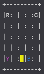
The output of env.render() represents the grid. The passenger is picked up and dropped off on one of the following: red(R), green(G), yellow (Y), and blue(B). In the image above, the passenger is on B (colored blue) and the passenger is on Y (colored magenta). If the taxi is full it is rendered green, otherwise it is yellow. This time, we do not need to create a separate method to run an episode; the agent is trained in each time step.

Here the agent is randomly selecting moves. Someday the taxi might reach its destination, but I wouldn't count on it.

SARSA Taxis

Let’s first use SARSA to train our agent. For the ϵ-greedy exploration policy, we implement a separate function.

def gen_eps_greedy_policy(num_actions, epsilon):
    # Epsilon Greedy exploratory policy 
    def policy_function(state, Q):
        probs = torch.ones(num_actions) * epsilon / num_actions
        best_action = torch.argmax(Q[state]).item()
        probs[best_action] += 1 - epsilon
        action = torch.multinomial(probs, 1).item()
        return action
    return policy_function

This form of function encapsulation is the same as what we did in the behavior policy generation function before. The probabilities are calculated and an action is selected from the multinomial distribution.

def sarsa(env, gamma, num_episodes, alpha, eps_policy):
    num_actions = env.action_space.n
    Q = defaultdict(lambda: torch.zeros(num_actions))
    for episode in tqdm(range(num_episodes)):
        state = env.reset()
        is_done = False
        action = eps_policy(state, Q)
        while not is_done:
            next_state, reward, is_done, info = env.step(action)
            next_action = eps_policy(next_state, Q)
            del_td = reward + gamma * Q[next_state][next_action] - Q[state][action]
            Q[state][action] += alpha * del_td
            state = next_state
            action = next_action
    policy = {}
    for state, actions in Q.items():
        policy[state] = torch.argmax(actions).item()
    return Q, policy

Here we run the simulation num_episodes number of times. In each time step of a simulation, we update the Q-function value for a state-action pair by alpha * del_td where del_td is the SARSA update. In the end we extract the optimal policy from the Q-function using torch.argmax.

Results

To visualize results, we first need a method to plot them. For this we will use matplotlib.

def plot_rate(episode_length, total_reward_episode):
    fig, ax = plt.subplots(1, 2, figsize=(12, 6))
    ax[0].plot(episode_length)
    ax[0].set_title("Episode Length over time")
    ax[0].set(xlabel="Episode", ylabel="Length")
    ax[1].plot(total_reward_episode)
    ax[1].set_title("Episode reward over time")
    ax[1].set(xlabel="Episode reward over time", ylabel="Reward")

    plt.show()

This is a very simple function that uses two subplots (labeled ax[0] and ax[1]) to visualize episode lengths and episode rewards.

On to running our algorithm.

num_episodes = 1000
episode_length = [0] * num_episodes
total_reward_episode = [0] * num_episodes

gamma = 1
alpha = 0.6
epsilon = 0.01        # Grid Search parameters
eps_policy = gen_eps_greedy_policy(env.action_space.n, epsilon)
optimal_Q, optimal_policy = sarsa(env, gamma, num_episodes, alpha, eps_policy)

plot_rate(episode_length, total_reward_episode)

γ is set to 1 because the previous action directly affects the next one. To find the best epsilon and gamma, you need to run the experiment many times. This part is mostly trial and error. Add the following lines within the while not is_done loop to make plots.

total_reward_episode[episode] += reward
episode_length[episode] += 1

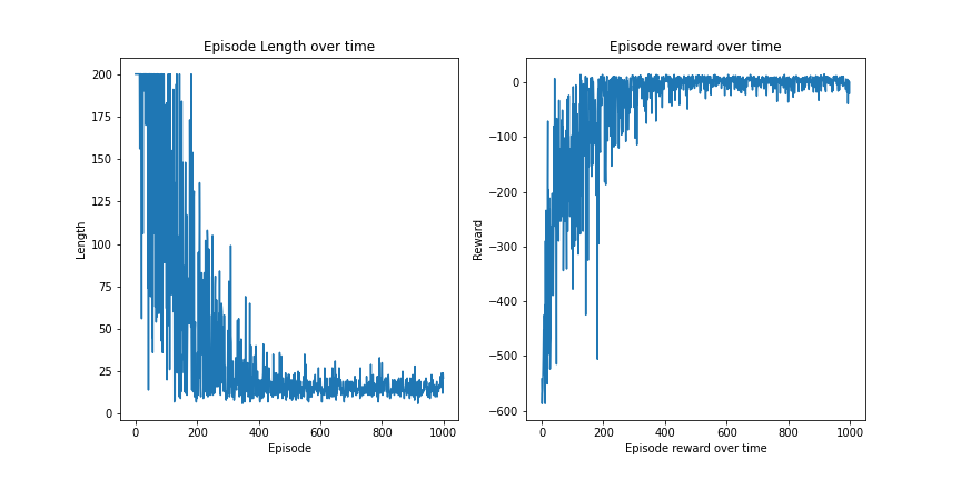
We then plot the results.

plot_rate(episode_length, total_reward_episode)

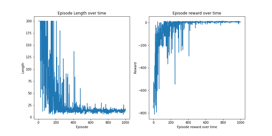
Episode length and reward over time for the SARSA algorithm in Taxi-v3. The policy stabilizes very well in 400 episodes.

SARSA works very well with the Taxi-v3 environment. The agent reaches the optimal policy by 400 episodes. There is some fluctuation as the passenger position is always random. The fact that we have the optimal hyperparameters should also be noted.

In summary, SARSA is great for the problem.

The agent following the SARSA optimal policy. See how few the number of moves are.

Q-Learning the Cab

Let’s now head over to Q-learning. We will again use the ϵ-greedy policy as our behavior policy.

These are our parameters. The episode_length and total_reward_episode arrays are required for visualizations.

num_episodes = 1000
episode_length = [0] * num_episodes
total_reward_episode = [0] * num_episodes

gamma = 1
alpha = 0.4
epsilon = 0.1
behaviour_policy = gen_eps_greedy_policy(env.action_space.n, epsilon)

On to the Q-learning algorithm.

def q_learning(env, behaviour_policy, gamma, num_episodes, alpha):
    num_actions = env.action_space.n
    Q = defaultdict(lambda: torch.zeros(num_actions))
    for episode in tqdm(range(num_episodes)):
        state = env.reset()
        is_done = False
        while not is_done:
            action = behaviour_policy(state, Q)
            next_state, reward, is_done, info = env.step(action)
            # Time step update
            del_td = reward + gamma * torch.max(Q[next_state]) - Q[state][action]   
            Q[state][action] += alpha * del_td
            state = next_state
            total_reward_episode[episode] += reward
            episode_length[episode] += 1
    policy = {}
    for state, actions in Q.items():
        policy[state] = torch.argmax(actions).item()
    return Q, policy

Notice the main difference in the two algorithms. Q-learning uses torch.max. This one line makes it off-policy because there is no guarantee we will be using the action output by torch.max in the next time step.

Results

Just like last time, we will be using the plot_rate method to plot the graphs.

plot_rate(episode_length, total_reward_episode)

Episode length and reward over time for the Q-learning algorithm in Taxi-v3. Although the policy stabilizes by 400 episodes, the fluctuations are larger.

As stated before, Q-learning is prone to weaker results due to its greedy nature. This is clearly visible here, as the fluctuations in rewards and lengths are larger than that of SARSA. An improvement to this is double Q-learning. Feel free to try that out with the algorithm given above. Double Q-learning is slower to learn because it uses two Q-functions at once. Increasing the number of episodes to 3000 will give good results.

Conclusion

Temporal difference learning contains some of the most powerful reinforcement learning algorithms we have seen yet. It is a concept that has its roots deep in RL. TD uses concepts from both Monte Carlo and reinforcement learning, making this strategy very versatile.

TD algorithms sample the expected value of V (MC sampling) and use this estimate to find the optimal value function (bootstrapping). This estimations on estimates may seem shaky, but due to the maximum-likelihood estimations the algorithms make, the results tend to be the most accurate.

In this article we looked at some of the main temporal difference learning algorithms. Starting from evaluation using TD(0) to control using SARSA and Q-learning, all TD algorithms use straightforward ways to solve problems. This makes TD algorithms easy to implement.

We also looked at Taxi-v3, a complex environment where the agent picks up and drops off passengers to and from random locations. This is the hallmark of a non-stationary problem. Some of the approaches we’d seen previously will most likely fail here, but temporal difference learning solves it easily. In fact, training takes about a minute in both the algorithms tried above.

Next time, we will look a bit more at temporal difference learning and number of hybrid methods that use a mix of the concepts seen before. Namely, the next article will be on TD(γ), tabular methods and the actor-critic model. Deep reinforcement learning robots aren’t far off!

Footnotes

[1] Sutton, R. S., & Barto, A. G. (2018). Reinforcement learning: An Introduction. MIT press.

[2] Watkins, C. J., & Dayan, P. (1992). Q-learning. Machine learning, 8(3-4), 279-292.

[3] Hasselt, H. (2010). Double Q-learning. Advances in neural information processing systems, 23, 2613-2621.